


Machine learning involves taking hundreds of thousands of data points and feeding them through a neural network, which then makes predictions about what the data is. In order to understand what machine learning is, it is important to understand the fundamentals, or in this case, neural networks. Computer Neural Networks are based on the human brain. When simulating our brains’ neural networks, we call it an “artificial neural network.” Our brains contain over ten billion neurons that are all connected to over ten thousand OTHER neurons. Each neuron then receives electrochemical signals from the other neurons, and when these signals are powerful enough, they activate the neurons! As these neurons are activated, they pass signals (messages) along to other neurons. There are many types of neural networks in machine learning, such as CNN’s and RNNs, but for this article, we will be focusing on the most basic neural network, the multilayer perceptron!
In a multilayer perceptron, a neuron is a value that holds a number between 0 and 1. This number corresponds to the color value of a pixel (when doing image recognition). A neuron is “activated” when it has a specific value that is larger than a threshold, much like neurons in the brain. Each pixel of an image make up the first layer of a neural network.
The last layer of a network is its output or the prediction it makes. The output layer can be a true or false, the prediction of what an object is (such as whether an image depicts a cat, a dog, or an elephant), etc… The number of neurons in the last layer is the number of possible outcomes. For the examples above, the number of neurons would be two and three respectively! The activation of these neurons corresponds to how confident the neural network is in its prediction. If a neural network was made to predict whether something is true or false, the activation could be .12 and .88 respectively.
The layers in between these two are called hidden layers. The number of neurons and hidden layers are variables based on user input, depending on what works best for the network.
All three layers interact the same way as a biological neural network, that is, each input is passed on to the next layer, and certain neurons are “fired.” These fired neurons fire neurons in the next layer, and this process is repeated until the final layer when a prediction is made. The neuron with the highest activation at the end is the prediction. But what is the goal of layers? The goal of layers is to optimize recognition. If one is detecting a dog, for example, we would hope that one layer recognizes the ears, one recognizes the nose, one recognizes the torso, and one recognizes the legs. Layers piece together components of an image to form a full image. The recognition of specific parts plays a role in the outcome. If each layer identifies one piece of a dog, we would hope that the output layer predicts “dog.” If one layer identifies a piece of a cat, however, the confidence of the output layer would be lower. Each layer continuously identifies a larger part of an image. The first layer may identify the curved edge of a dog ear, whereas the second layer identifies the entire dog ear. This layering is known as “abstraction.”
So, how does a layer look for a certain pattern? Each input neuron is connected to a weight, which can be changed by the user or through other algorithms (ex. backpropagation). In a neural network, weights are what need to be altered to gain accuracy. To represent this mathematically, we must take the weighted sum, and multiple each activation with its corresponding weight (a1w1+a2w2+…+anwn). To enable a layer to look for a certain pattern, such as the tip of a dog ear, we can set all weight values to 0 besides weight values in the region we are interested in. This way, we will only get positive activation values for the region we are interested in. Recall that activations must be a number between 0 and 1. Because the weighted sum could be anywhere on the number line, we must have some sort of function to ensure that all values are in the 0-1 range. There are many functions that can do this, including the sigmoid function (1/1+e^-x). The sigmoid function allows negative sums to be close to zero and positive sums are close to one.

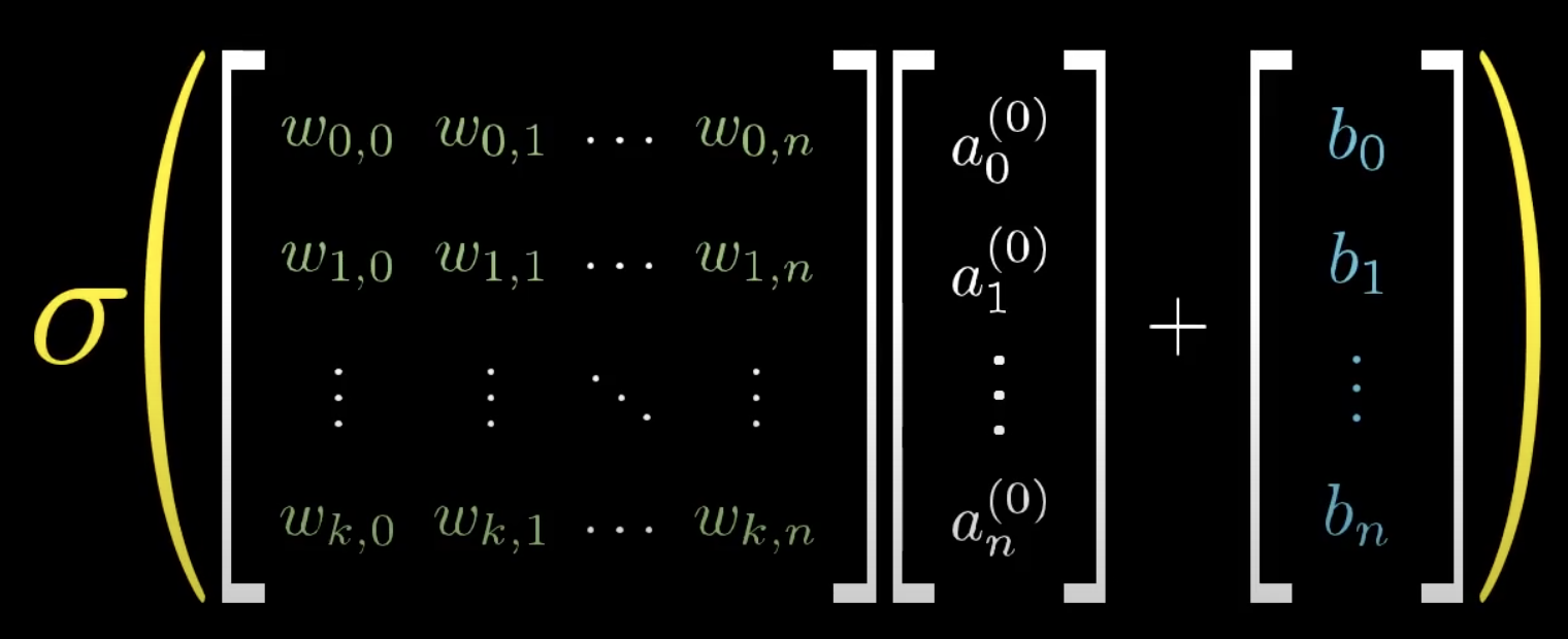
There are many activation functions that can do the same task, such as ReLU, Leaky ReLU, ELU, TanH, and many more. After applying an activation function, our new equation is activation(a1w1+a2w2+…+anwn), for sigmoid, it is σ(a1w1+a2w2+…+anwn). Essentially, this new sum indicates how positive the activation is, or how “fired” it is. We can set some sort of threshold to indicate how “activated” a function must be to actually “fire up” and set off a neuron in the next layer. This number can change based on the network, however, in its most basic form, this threshold is zero. If we want to set this threshold to a higher number, such as zero, we must apply a “bias.” Before the network is manipulated by the nonlinear activation function, we can add or subtract a bias. If I want my threshold to be 10, my equation will now look like σ(a1w1+a2w2+…+anwn-10), or in general terms, σ(a1w1+a2w2+…+anwn+b). When reading up more about neural networks, you will probably see this equation in the form of a matrix, that is, each activation is in a vector with one column and n number of rows. Another matrix contains all of the weights, with n rows and n columns (same number of columns as the activation matrix). The dot product of these two is taken. Then, a vector containing all of the biases is added to this dot product. Finally, it is multiplied by a nonlinear activation function. This can then be simplified even further into: a=σ(Wa+b)
To summarize the above paragraphs, the weight indicates which pattern a neuron is looking for, and the bias indicates how high the threshold must be for a neuron to be meaningfully active, or high enough to be actually useful. Each neuron from the first layer is connected to each neuron from the second layer. Each previous layer is connected to the layer after it, which is a lot of layers to even think about! Each layer is also connected to its own set of weights and biases, which means that there are an immense amount of neurons AND connections in a neural network, much like your own brain.
This large number of connections leads to one issue… there are an immense amount of weights and biases that can be tweaked to have a high performing network. The learning aspect of machine learning only refers to the tweaking of these weights and biases, and lucky for us, we can force our machine learning models to do this for us (it is called machine learning, after all)! This is done in multiple steps. The first step is identifying how “correct” the output layer was. We compare the actual result with the expected result and find the squares of the differences (for example, a network might have activation of .73 for true and .27 for false, but the expected result would be 1.00 for true and .00 for false). We then take the average “correctness,” also known as “cost,” among all the data, which is a measure for how good (or bad), a network is.
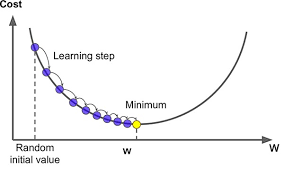
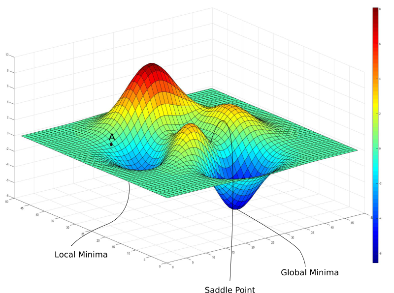
The next thing we need to do is teach the machine learning network how to get better, because (unfortunately), just telling it how good or bad it is won’t increase the accuracy of the network. To do this, we must identify a function that minimizes the cost. On a graph, this would look like the lowest “dip,” and is known as the minimum (just think of the cost function as c(w)). To get to the lowest dip, we can start at a random location on the graph (a randomly generated weight), and then move left or right depending on whether the slope of that point is positive or negative (respectively). If we continue to do this, at some point, we will get to the lowest point on the graph, similar to a ball rolling down a hill. There is one issue with this, however. Imagine if we had a graph with many dips, such as the one displayed here. Depending on where we randomize our weights, we might reach different local minima. Because of this, we never know whether we are truly at the lowest point on the graph. Lucky for us, we can identify the “gradient,” or the direction of the steepest increase using multivariable calculus. We can take the negative of this gradient and go in the steepest downward direction! We can apply the values given to us by the gradient to nudge the weights and biases, therefore taking us to the local minima. As we keep editing the cost function, we will notice that it starts to look less random and that there is a significant increase in accuracy (for reference, rather than having a .72 and .23 prediction, we might have a .98 and .02 prediction for true and false respectively)! When a network learns, we are simply talking about decreasing the cost function. The above paragraph describes the “gradient descent function.” Essentially, this function denotes the importance of each weight and bias and increases the most important ones while decreasing the least important ones.
After identifying which directions the weights and biases have to go in, we must reprocess them such that we can go back to the beginning of the network and actually adjust the weights and biases. This process is known as backpropagation, and I urge you to look into backpropagation algorithms! For now, you’ve mastered the mathematics behind forwarding propagation in the multilayer perceptron!


